Maven02

Maven Market Project - Analyzing Data of a Grocery Chain Firm

Introduction

This Project Case is part of the Microsoft Power BI Desktop for Business Intelligence Course on Udemy online platform by Maven Analytics. In this case, I am being put in the point of view of a Business Intelligence Analyst in Maven Market, a Multinational Grocery Chain company whose business locations are in Canada, Mexico and the United States. My role is to transform raw data into a dashboard report to help the Management Team track the KPI, monitor and compare the performance, as well as identify some insights. I worked through the entire business intelligence workflow, i.e.: connecting and shaping the data, building a relational model, adding calculated fields, and designing an interactive report.

Problem Questions

The Management Team would like to find out the Topline Performance of their products. This must be delivered by:

Defining the Top 30 Product Brands with highest Total Transactions and their corresponding Profit, Profit Margin, as well as Return Rate in descending order.
Providing KPI information displaying the Current Month Transactions vs Last Month Transactions, Current Month Profit vs Last Month Profit, and Current Month Returns vs Last Month Returns.
Displaying a visual geographical map showing Transactions by Cities in which the company stores are operating.
Providing information of Total Transaction in each of the country that can be drilled up/down, so that the granularity of the information can be determined in either level of country, city, or state.
Providing the weekly trending of the company’s revenue, especially during the year 1998. Besides that, the management also wanted to find out the highest monthly revenue ever achieved.

Datasets

There are 7 Datasets used in this project, i.e.:

1. Customer Table Dataset (MavenMarket_Customers.csv)

Field Name	Data Type
customer_id	Whole Number
customer_acct_num	Text
first_name	Text
last_name	Text
customer_address	Text
customer_city	Text
customer_state_province	Text
customer_postal_code	Text
customer_country	Text
birthdate	Date
marital_status	Text
yearly_income	Text
gender	Text
total_children	Whole Number
num_children_at_home	Whole Number
education	Text
acct_open_date	Date
member_card	Text
occupation	Text
homeowner	Text
full_name	Text
birth_year	Text
has_children	Y/N

2. Products Table Dataset (MavenMarket_Products.csv)

Field Name	Data Type
product_id	Whole Number
product_brand	Text
product_name	Text
product_sku	Text
product_retail_price	Decimal Number
product_cost	Decimal Number
product_weight	Decimal Number
recyclable	Decimal Number
low_fat	Decimal Number
discount_price	Fixed Decimal Number (Currency)

3. Calendar Table Dataset (MavenMarket_Calendar.csv)

Field Name	Data Type
date	Date
Start of Week	Date
Name of Day	Text
Start of Month	Date
Name of Month	Text
Quarter	Whole Number
Year	Whole Number

4. Regions Table Dataset (MavenMarket_Regions.csv)

Field Name	Data Type
region_id	Whole Number
sales_district	Text
sales_region	Text

5. Stores Table Dataset (MavenMarket_Stores.csv)

Field Name	Data Type
store_id	Whole Number
region_id	Whole Number
store_type	Text
store_name	Text
store_street_address	Text
store_city	Text
store_state	Text
store_country	Text
store_phone	Text
first_opened_date	Date
last_remodel_date	Date
total_sqft	Whole Number
grocery_sqft	Whole Number
full_address	Text
area_code	Text

6. Transaction Table Dataset (MavenMarket_Transactions_1997 & MavenMarket_Transactions_1998.csv)

Field Name	Data Type
transaction_date	Date
stock_date	Date
product_id	Whole Number
customer_id	Whole Number
store_id	Whole Number

7. Return Table Dataset (MavenMarket_Returns_1997-1998.csv)

Field Name	Data Type
return_date	Date
product_id	Whole Number
store_id	Whole Number
quantity	Whole Number

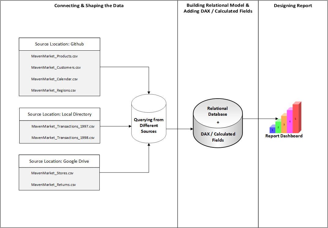
Connecting and Shaping the Data

There are several steps in this phase in order to connect and shape the Data used in this case.

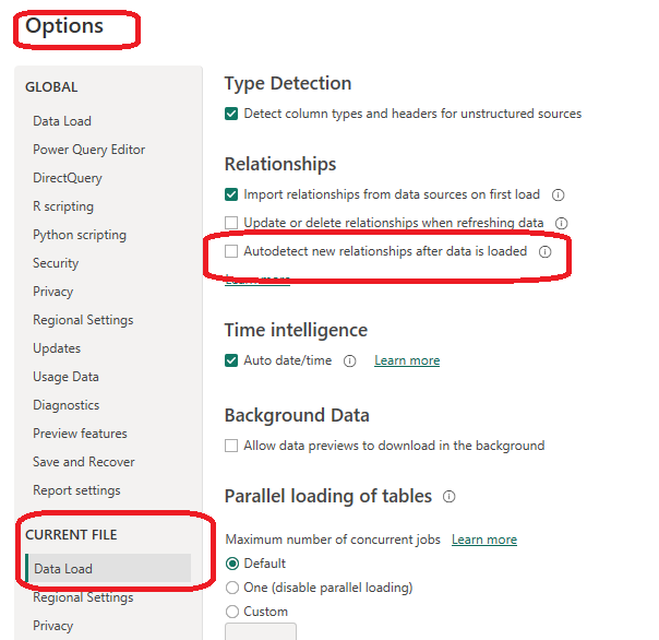
1. Update Power BI options and settings by:

Deselecting the “Autodetect new relationships after data is loaded” option in the Data Load tab
Making sure that Locale for import is set to “English (United States)” in the Regional Settings tab

2. Connect to the MavenMarket_Customers csv file by:

Naming the table “Customers”, and making sure that headers have been promoted
Confirming that data types are accurate (Note: “customer_id” should be whole numbers, and both “customer_acct_num” and “customer_postal_code” should be text)
Adding a new column named “full_name” to merge the the “first_name” and “last_name” columns, separated by a space
Creating a new column named “birth_year” to extract the year from the “birthdate” column, and format as text
Creating a conditional column named “has_children” which equals “N” if “total_children” = 0, otherwise “Y”

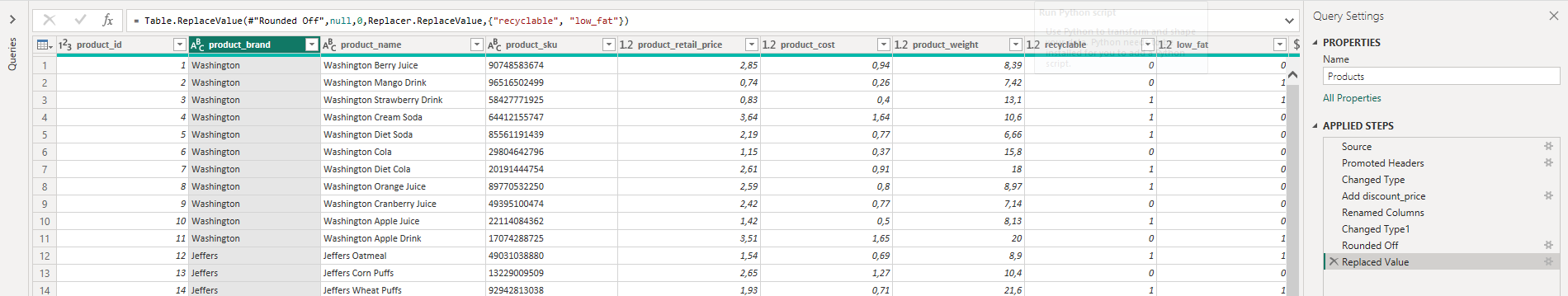
3. Connect to the MavenMarket_Products csv file by:

Naming the table “Products” and making sure that headers have been promoted
Confirming that data types are accurate (Note: “product_id” should be whole numbers, “product_sku” should be text), “product_retail_price” and “product_cost” should be decimal numbers)
Using the statistics tools to return the number of distinct product brands, followed by distinct product names and conducting Spot check to see 111 brands and 1,560 product names
Adding a calculated column named “discount_price”, equal to 90% of the original retail price and formating as a fixed decimal number, and then use the rounding tool to round to 2 digits
Selecting “product_brand” and use the Group By option to calculate the average retail price by brand, and name the new column “Avg Retail Price”. Conducting Spot check to see an average retail price of $2.18 for Washington products, and $2.21 for Green Ribbon
Deleting the last applied step to return the table to its pre-grouped state
Replacing “null” values with zeros in both the “recyclable” and “low-fat” columns

4. Connect to the MavenMarket_Stores csv file by:

Naming the table “Stores” and making sure that headers have been promoted
Confirming that data types are accurate (Note: “store_id” and “region_id” should be whole numbers)
Adding a calculated column named “full_address”, by merging “store_city”, “store_state”, and “store_country”, separated by a comma and space (hint: use a custom separator)
Adding a calculated column named “area_code”, by extracting the characters before the dash (“-“) in the “store_phone” field

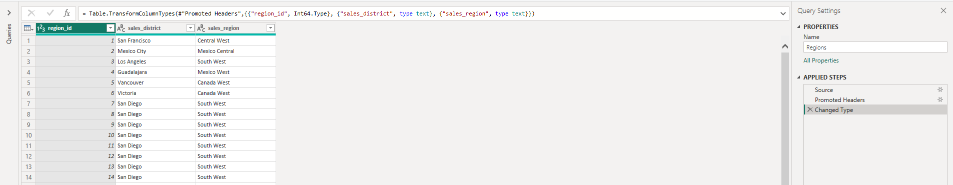
5. Connect to the MavenMarket_Regions csv file by:

Naming the table “Regions” and making sure that headers have been promoted
Confirming that data types are accurate (Note: “region_id” should be whole numbers)

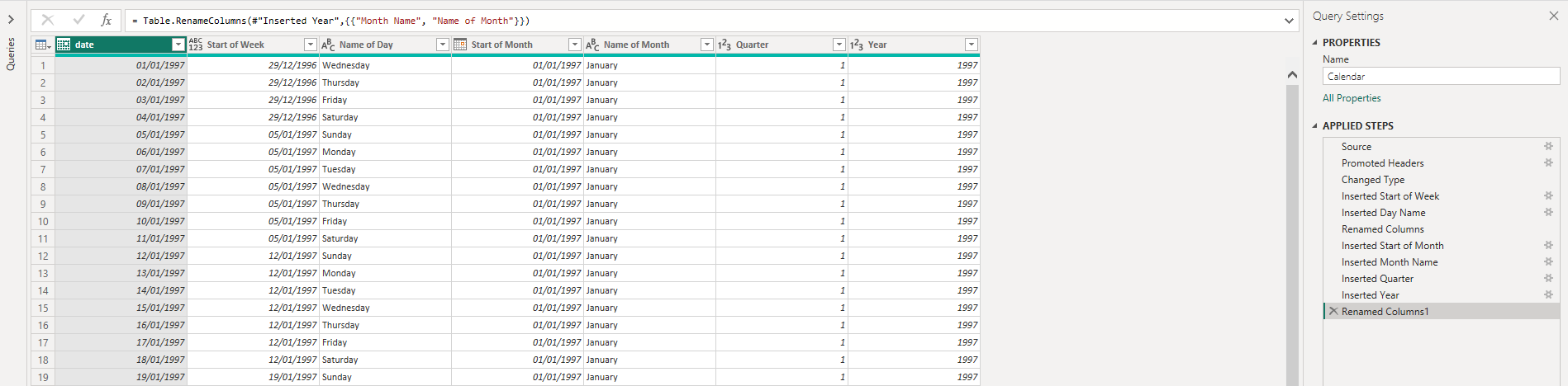
6. Connect to the MavenMarket_Calendar csv file by:

Naming the table “Calendar” and making sure that headers have been promoted
Using the date tools in the query editor to add the following columns:

Start of Week, Name of Day, Start of Month, Name of Month, Quarter of Year, Year

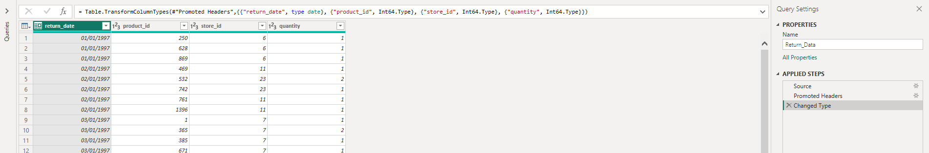
7. Connect to the MavenMarket_Returns csv file by:

Naming the table “Return_Data” and making sure that headers have been promoted
Confirming that data types are accurate (all ID columns and quantity should be whole numbers)

8. Add a new folder on your desktop (or in your documents) named “MavenMarket Transactions”, containing both the MavenMarket_Transactions_1997 and MavenMarket_Transactions_1998 csv files by:

Connecting to the folder path, and choosing “Edit” (vs. Combine and Edit)
Clicking the “Content” column header (double arrow icon) to combine the files, then removing the “Source.Name” column
Naming the table “Transaction_Data”, and confirming that headers have been promoted
Confirming that data types are accurate (all ID columns and quantity should be whole numbers) and conducting Spot check to see data from 1/1/1997 through 12/30/1998 in the “transaction_date” column

9. With the exception of the two data tables, disable “Include in Report Refresh”, then Close & Apply by:

Confirming that all 7 tables are now accessible within both the RELATIONSHIPS view and the DATA view

Building a Relational Model

There are several steps in this phase in order to build a Relational Model.

1. In the MODEL view, arrange the tables so that the lookup tables are above the data tables by:

Connecting Transaction_Data to Customers, Products, and Stores using valid primary/foreign keys
Connecting Transaction_Data to Calendar using both date fields, with an inactive “stock_date” relationship
Connecting Return_Data to Products, Calendar, and Stores using valid primary/foreign keys
Connecting Stores to Regions as a “snowflake” schema

2. Confirm the following:

All relationships follow one-to-many cardinality, with primary keys (1) on the lookup side and foreign keys (*) on the data side
Filters are all one-way (no two-way filters)
Filter context flows “downstream” from lookup tables to data tables
Data tables are connected via shared lookup tables (not directly to each other)

3. Hide all foreign keys in both data tables from Report View, as well as “region_id” from the Stores table

4. In the DATA view, complete the following steps by:

Updating all date fields (across all tables) to the “M/d/yyyy” format using the formatting tools in the Modeling tab
Updating “product_retail_price”, “product_cost”, and “discount_price” to Currency ($ English) format
In the Customers table, categorizing “customer_city” as City, “customer_postal_code” as Postal Code, and “customer_country” as Country/Region
In the Stores table, categorizing “store_city” as City, “store_state” as State or Province, “store_country” as Country/Region, and “full_address” as Address

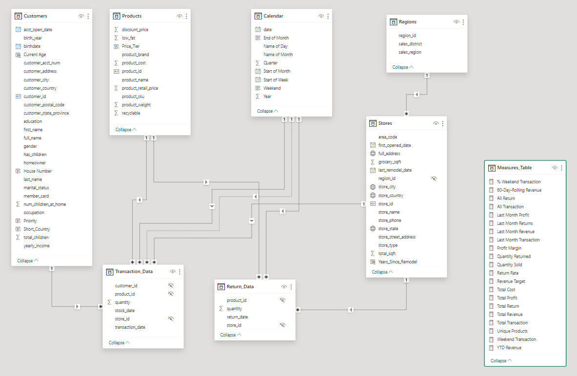
All the steps above resulted in the following Relation Model:

Adding Calculated Fields and DAX (Data Analysis eXpression)

There are 2 spots in which I worked to add Calculation Fields and DAX, i.e. the Data View and the Report View.

1. In the DATA view, add the following calculated columns by:

Adding a column in the Calendar table, named “Weekend”, which equals “Y” for Saturdays or Sundays (otherwise “N”)
```
Weekend = 
if('Calendar'[Name of Day] IN {"Saturday","Sunday"},"Y","N")
```
Adding a column in the Calendar table, named “End of Month”, that returns the last date of the current month for each row
```
End of Month = EOMONTH('Calendar'[date],0)
```
Adding a column in the Customers table, named “Current Age” that calculates current customer ages using the “birthdate” column and the TODAY() function
```
Current Age = DATEDIFF(Customers[birthdate], TODAY(), YEAR)
```
Adding a column in the Customers table, named “Priority” which equals “High” for customers who own homes and have Golden membership cards (otherwise “Standard”)
```
Priority = IF(Customers[homeowner]="Y" && Customers[member_card]="Golden","High","Standard")
```
Adding a column in the Customers table, named “Short_Country” that returns the first three characters of the customer country, and converts to all uppercase
```
Short_Country = UPPER(LEFT(Customers[customer_country],3))
```
Adding a column in the Customers table, named “House Number” that extracts all characters/numbers before the first space in the “customer_address” column (hint: use SEARCH)
```
House Number = LEFT(Customers[customer_address],SEARCH(" ",Customers[customer_address])-1)
```
Adding a column in the Products table, named “Price_Tier” that equals “High” if the retail price is >$3, “Mid” if the retail price is >$1, and “Low” otherwise
```
Price_Tier = SWITCH(TRUE(),Products[product_retail_price]>3,"High",Products[product_retail_price]>1,"Mid","Low")
```
Adding a column in the Stores table, named “Years_Since_Remodel” that calculates the number of years between the current date (TODAY()) and the last remodel date
```
Years_Since_Remodel = DATEDIFF(Stores[last_remodel_date],TODAY(),YEAR)
```

2. In the REPORT view, add the following measures (Assign to tables as you see fit, and use a matrix to match the “spot check” values) by:

Creating new measures named “Quantity Sold” and “Quantity Returned” to calculate the sum of quantity from each data table, and conducting Spot check to see total Quantity Sold = 833,489 and total Quantity Returned = 8,289
```
Quantity Sold = SUM(Transaction_Data[quantity])
Quantity Returned = SUM(Return_Data[quantity])
```
Creating new measures named “Total Transactions” and “Total Returns” to calculate the count of rows from each data table, and conducting Spot check to see 269,720 transactions and 7,087 returns
```
Total Transaction = COUNTROWS(Transaction_Data)
Total Return = COUNT(Return_Data[return_date])
```
Creating a new measure named “Return Rate” to calculate the ratio of quantity returned to quantity sold (format as %), and conducting Spot check to see an overall return rate of 0.99%
```
Return Rate = DIVIDE([Quantity Returned],[Quantity Sold])
```
Creating a new measure named “Weekend Transactions” to calculate transactions on weekends, and conducting Spot check to see 76,608 total weekend transactions
```
Weekend Transaction = CALCULATE([Total Transaction],'Calendar'[Weekend]="Y")
```
Creating a new measure named “% Weekend Transactions” to calculate weekend transactions as a percentage of total transactions (format as %), and conducting Spot check to see 28.4% weekend transactions
```
% Weekend Transaction = DIVIDE([Weekend Transaction],[Total Transaction])
```
Creating new measures named “All Transactions” and “All Returns” to calculate grand total transactions and returns (regardless of filter context), and conducting Spot check to see 269,720 transactions and 7,087 returns across all rows
```
All Transaction = CALCULATE([Total Transaction],ALL(Transaction_Data))
All Return = CALCULATE([Total Return],ALL(Return_Data))
```
Creating a new measure to calculate “Total Revenue” based on transaction quantity and product retail price, and formating as $ (using and iterator), as well as conducting pot check to see a total revenue of $1,764,546
```
Total Revenue = SUMX(Transaction_Data,Transaction_Data[quantity]*RELATED(Products[product_retail_price]))
```
Creating a new measure to calculate “Total Cost” based on transaction quantity and product cost, and formating as $ (using an iterator), as well as conducting Spot check to see a total cost of $711,728
```
Total Cost = SUMX(Transaction_Data,Transaction_Data[quantity]*RELATED(Products[product_cost]))
```
Creating a new measure named “Total Profit” to calculate total revenue minus total cost, formating as $, and conducting Spot check to see a total profit of $1,052,819
```
Total Profit = [Total Revenue]-[Total Cost]
```
Creating a new measure to calculate “Profit Margin” by dividing total profit by total revenue calculate total revenue (format as %), and conducting Spot check to see an overall profit margin of 59.67%
```
Profit Margin = DIVIDE([Total Profit],[Total Revenue])
```
Creating a new measure named “Unique Products” to calculate the number of unique product names in the Products table, and conducting Spot check to see 1,560 unique products
```
Unique Products = DISTINCTCOUNT(Products[product_name])
```
Creating a new measure named “YTD Revenue” to calculate year-to-date total revenue, formating as $, and createing a matrix with “Start of Month” on rows to see $872,924 in YTD Revenue in September 1998 for Spot check
```
YTD Revenue = CALCULATE([Total Revenue],DATESYTD('Calendar'[date]))
```
Creating a new measure named “60-Day Rolling Revenue” to calculate a running revenue total over a 60-day period, formating as $, and creating a matrix with “date” on rows to see $97,570 in 60-Day Revenue on 4/14/1997 for Spot check
```
60-Day-Rolling Revenue = CALCULATE([Total Revenue],DATESINPERIOD ('Calendar'[Date],MAX('Calendar'[Date]),-60,DAY))
```

Creating new measures named “Last Month Transactions”, “Last Month Revenue”, “Last Month Profit”, and “Last Month Returns”, and creating a matrix with “Start of Month” on rows to confirm accuracy for Spot check

Last Month Transaction = CALCULATE([Total Transaction],DATEADD('Calendar'[date],-1,MONTH))
Last Month Revenue = CALCULATE([Total Revenue],DATEADD('Calendar'[Date],-1,MONTH))
Last Month Profit = CALCULATE([Total Profit],DATEADD('Calendar'[Date],-1,MONTH))
Last Month Returns = CALCULATE([Total Return],DATEADD('Calendar'[Date],-1,MONTH))

Creating a new measure named “Revenue Target” based on a 5% lift over the previous month revenue, and formating as $, and conducting Spot check to see a Revenue Target of $99,223 in March 1998
```
Revenue Target = [Last Month Revenue]*1.05
```

Executing all the detailed Steps in 2 spots above, resulted in adding a new Table containing all Measures needed in the modelling.

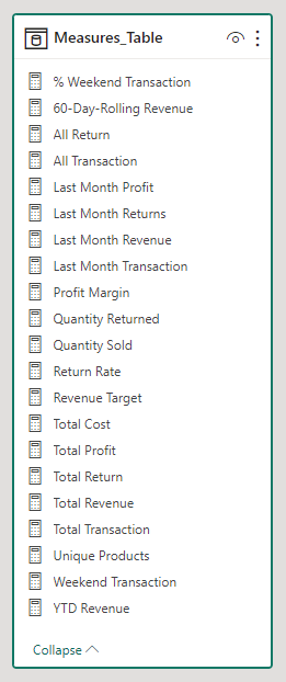
The overall tables created the complete Relation Model for all the data loaded in the Power Bi

Building Interactive Report

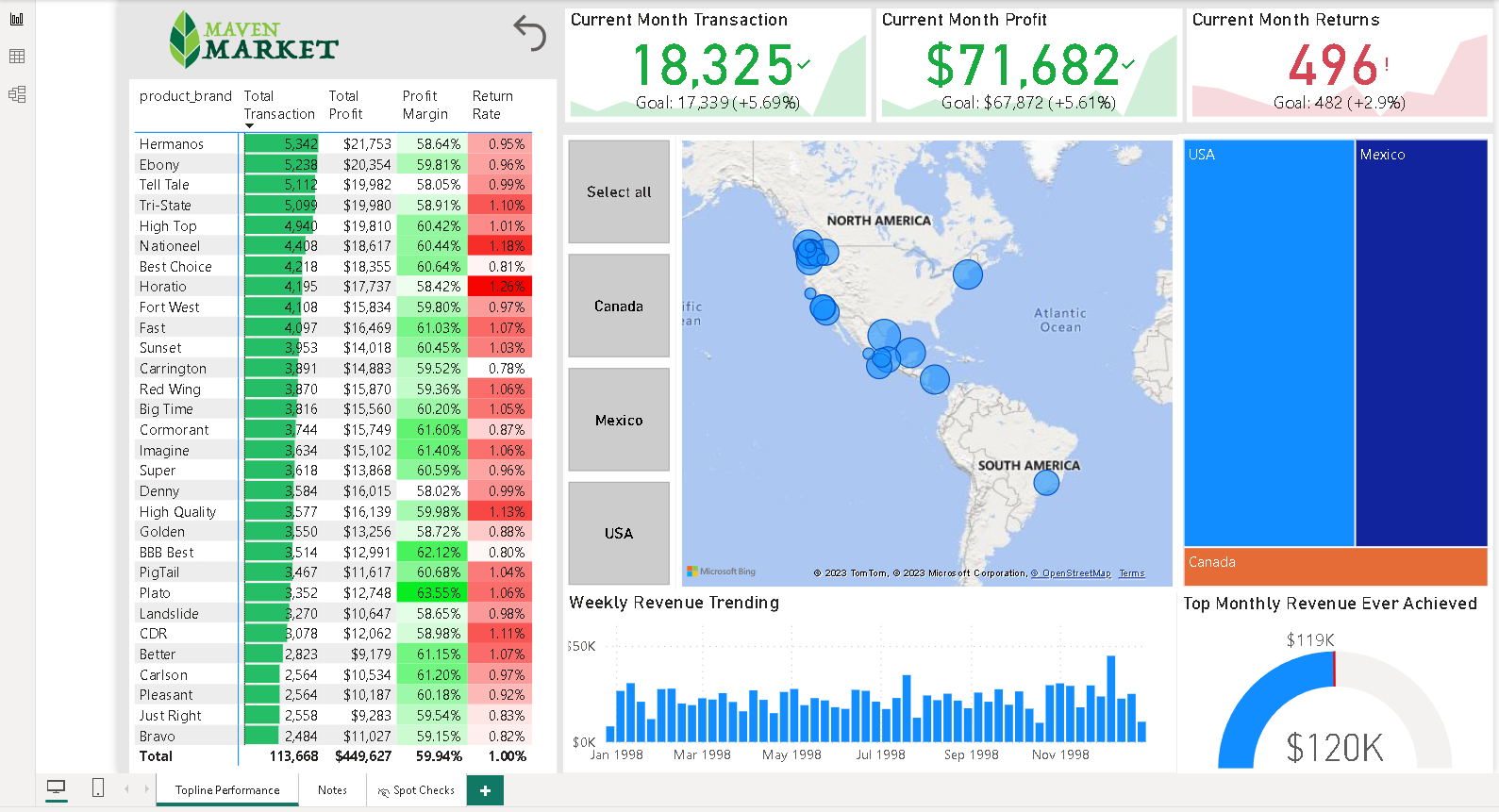
The report dashboard is to provide information in the Problem Questions Section. Below is the Dashboard for the report.

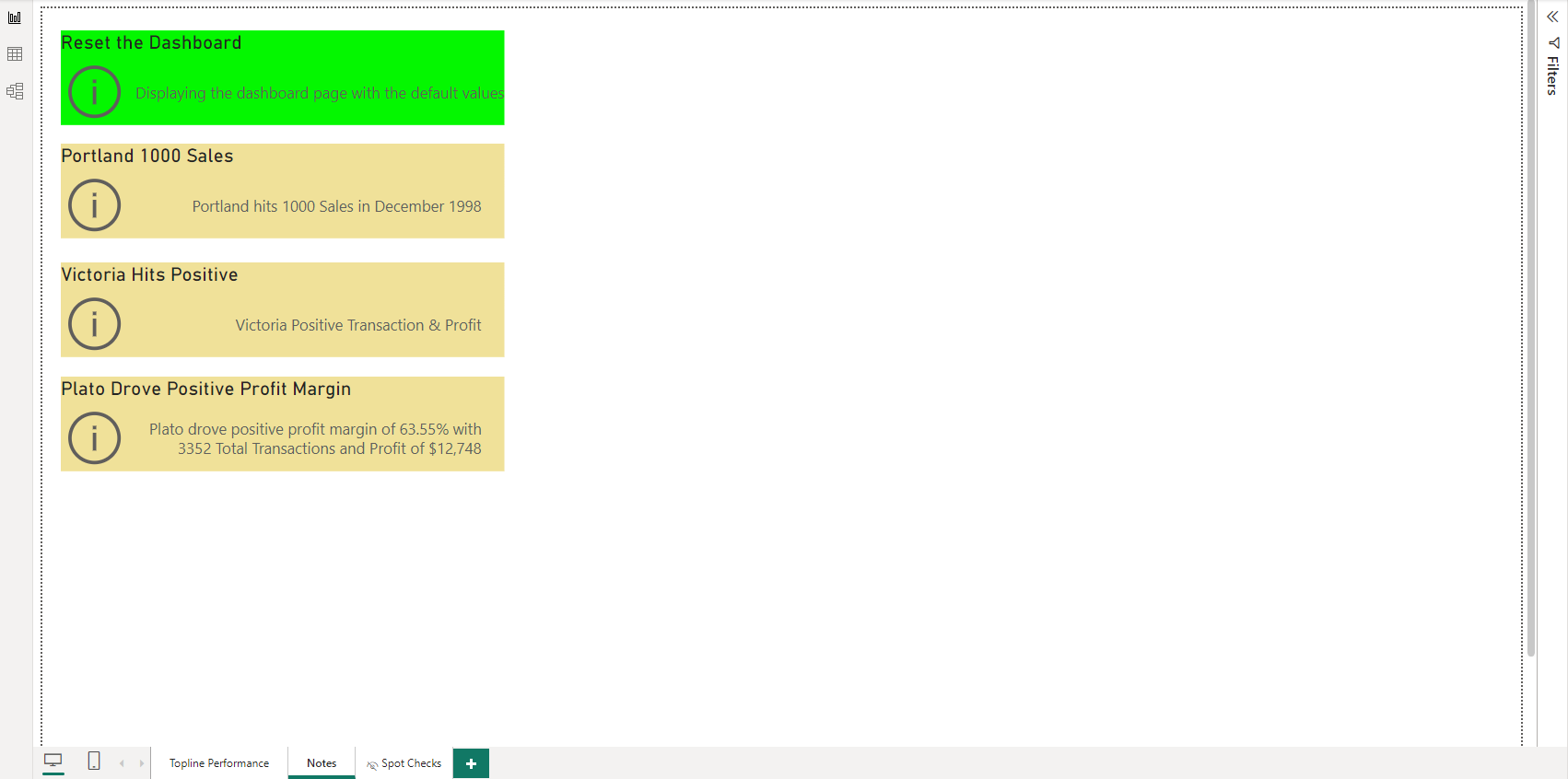
I also built a Note Report Page where its purpose is to provide insights (by utilizing the Bookmark function) so that it can be quickly shown to the management / stakeholders. Later on, for future use, I can add as many insights as can be found based on the data. Yet, in this case I only provided 3 quick insights, i.e.: Portland 1000 Sales, Victoria Hits Positive, and Plato drove the highest profit rate.

Analysis to answer the Problem Questions

Defining the Top 30 Product Brands with most Total Transactions and their corresponding Profit, Profit Margin, as well as Return Rate in descending order.

Solution:

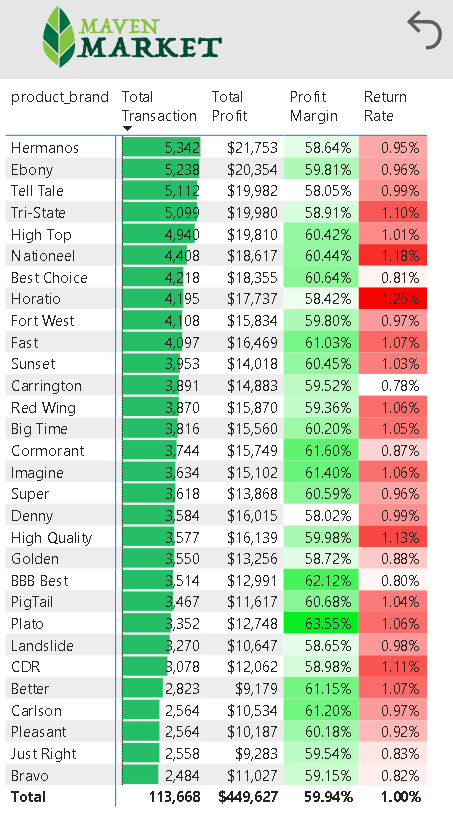
Based on the picture above, Hermanos peaked the position of the Top 30 Product Brands with the most Total Transaction of 5,342 with Total Profit of $ 21,753 and Margin of 58.64%, as well as Return Rate of 0.95%. Its position is followed by Ebony and Tell Tale in the second and third position. All the Top 30 Product Brand drove a total of 113,668 Transactions, with acumulative Profit Margin of 59.94% that equals to Total Profit of $ 449,627, and total Return Rate of 1.00%.

Providing KPI information displaying the Current Month Transactions vs Last Month Transactions, Current Month Profit vs Last Month Profit, and Current Month Returns vs Last Month Returns.

Solution:

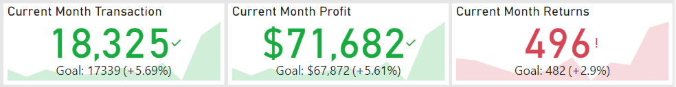
Based on the scorecards displayed above, the Total Transactions in the current month had reached 18,325 number of transaction. This has surpassed the target of 17,339 transaction (around 5.69% increment) above the last month transaction. This drove a 5.61% increment of profit which equals of a Total Profit of $ 71,682 in the current month. However, it turned out that in the same period, the current Monthly Returned also increased by 2.9% or equals 14 additional returns from the previous month return (482). This means along with the increasing number of transaction, there was also an increasing number of goods returned. It is advisable to examine the cause as well of the type of the returned goods.

Displaying a visual geographical map showing Transactions by Cities in which the company stores are operating.

Solution:

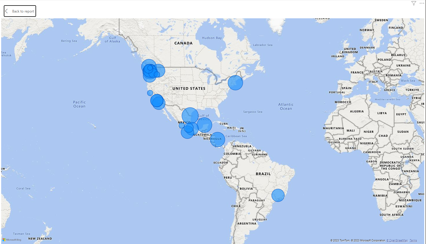
If we expand the map on the Dashboard, we will see from the map above that most of the stores are located in USA, while the country with the second most store number is Mexico. Canada is in the 3rd place for number of store in the country. This number of store drove the number of transaction, as well as total profit gained (representated by the bubble size).

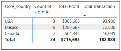
A quick spot check for Total Transactions and Total Profit for each country has confirmed that.

Providing information of Total Transaction in each of the country that can be drilled up/down, so that the granularity of the information can be determined in either level of country, city, or state.

Solution:

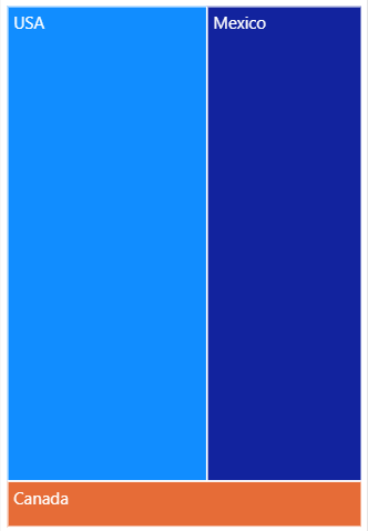
The Treemap above implies that most of the Transaction happened in the USA. This is because most stores are located in USA. This is aligned with the information provided in the previous solution. The more stores are open, the more Transaction will take place, which eventually would drive the Total Profit.

Providing the weekly trending of the company’s revenue, especially during the year 1998. Besides that, the management also wanted to find out the highest monthly revenue ever achieved.

Solution:

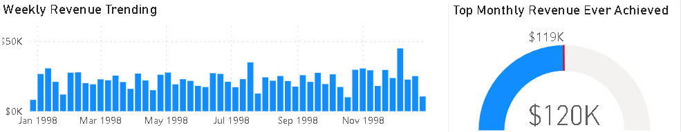
Based on the visuals above, the revenue experienced fluctuation over the time during year 1998. The highest revenue ever achieved was $ 120K, a slightly different from the corresponding target of around $ 119K.

Report Dashboard Link:

The live report dashboard can be found here